Tutorials

The atomic pair distribution function (PDF) provides a powerful route to understanding the local atomic structure of materials in real space. Despite its utility, PDF fitting and analysis can be challenging. The process of understand PDFs requires time, care, and the development of intuition to connect structural models to experimental data. Hopefully by the end of this tutorial series, PDF fitting will go from being a mysterious black box to a powerful tool in your structural analysis.

Example usage of diffpy.cmi can be found at this GitHub repo.

Structural parameters

Before we start fitting PDFs, lets first understand the parameters that will be refined on and what they mean. It is important to understand these parameters as they will help you gain better insight into the fitting process and how to interpret the results.

PDF Parameter	Description	Refineable?	Structural or Instrumental?
`a`, `b`, `c`	Lattice parameters of the crystal structure.	Yes	Structural
`alpha`, `beta`, `gamma`	Angles between lattice vectors	Yes	Structural
`delta1`	Constant (r-independent) peak broadening parameter accounting for uniform broadening of PDF peaks due to static disorder or residual instrumental effects.	Yes	Both
`delta2`	Correlated motion parameter accounting for r-dependent broadening (increases with r) of PDF peaks due to correlated atomic motion.	Yes	Structural
`biso` or `Uiso`	Isotropic atomic displacement parameter (ADP); models thermal vibration/disorder for each atom type. (note: `biso=8pi^2Uiso`)	Yes	Structural
`uij`	Anisotropic ADPs constrained by space group symmetry.	Yes	Structural
`dscale`	Correction factor for background or density mismatch.	Sometimes; often fixed	Instrumental
`sratio`	Ratio of coherent to incoherent scattering, used in some models.	Sometimes	Instrumental

Dataset parameters

PDF Parameter	Description	Refineable?	Structural or Instrumental?
`scale`	Overall scaling factor between calculated and observed PDFs; sets the absolute intensity.	Yes	Instrumental
`qdamp`	Damping of PDF peaks due to limited experimental Q-range. Typically affects high-r ripples and overall peak amplitudes.	Yes	Instrumental
`qbroad`	Instrumental or sample-related broadening of PDF peaks. This is due to the fact that diffraction peaks have different widths as a function of Q.	Yes	Instrumental
`qmin`	Minimum Q included in the fit; sets the lower bound of the fourier transform (converting S(Q) to G(r)).	No, from experiment/setup	Instrumental
`qmax`	Maximum Q included in the fit; sets the upper bound of the fourier transform (converting S(Q) to G(r)).	No, from experiment/setup	Instrumental
`rmin`	Minimum r (distance) included in the fit; sets the lower bound of the fitting range.	No, from experiment/setup	Instrumental
`rmax`	Maximum r (distance) included in the fit; sets the upper bound of the fitting range.	No, from experiment/setup	Instrumental (unless fitting to nanoparticles)

Bulk Ni PDF fitting

Although it is easier (and recommended) to fit PDFs of bulk homogeneous materials in PDFgui, fitting a bulk PDF in diffpy.cmi will provide you with a deeper insight into the fitting process. Additionally, this pedagogical example will help you build up confidence in using diffpy.cmi.

For bulk PDFs, we highly recommend using PDFgui. PDFgui is a great stepping stone before using diffpy.cmi. If you don’t know how to use PDFgui, please see this PDFgui tutorial to fit the same Ni PDF with PDFgui.

Data Download

First, visit this link and download the files for this tutorial:

Ni.cif
Ni.gr

To start, we must first import all necessary modules and packages.

import matplotlib.pyplot as plt
import numpy as np

from diffpy.utils.parsers.loaddata import loadData
from diffpy.structure import loadStructure
from diffpy.srfit.fitbase import FitContribution, FitRecipe
from diffpy.srfit.fitbase import Profile
from diffpy.srfit.pdf import PDFParser, PDFGenerator
from diffpy.structure.parsers import getParser
from diffpy.srfit.structure import constrainAsSpaceGroup

As a sanity check, lets load the cif and PDF data to see what they look like.

stru_path = "~/path/to/data/Ni.cif"
data_path = "~/path/to/data/Ni.gr"
# Load the structure and PDF data
structure = loadStructure(stru_path)
pdf_data = loadData(data_path)
print("Ni cif file:")
print(structure)

r = pdf_data[:, 0]
g = pdf_data[:, 1]
plt.plot(r, g, label="PDF Data")
plt.xlabel("r (Angstrom)")
plt.ylabel("G(r)")
plt.title("Ni PDF Data")
plt.legend()
plt.show()

Once you see the data and have a feel for it, we can begin the fitting process. We will first define the Dataset parameters and Structural parameters. These values will be used to initialize our fit. Given this data, these values are reasonable starting points.
```
PDF_RMIN = 1.5
PDF_RMAX = 50
PDF_RSTEP = 0.01
QMAX = 25
QMIN = 0.1
CUBICLAT_I = 3.52
SCALE_I = 0.4
UISO_I = 0.005
DELTA2_I = 2
QDAMP_I = 0.04
QBROAD_I = 0.02
```

Now, we will define a function called make_recipe. This function will essentially tell the fit what to do. It contains all the necessary parameters and contributions for the PDF fitting process. Because looking at a function with a lot of code is scary, here is a gist of what the function does.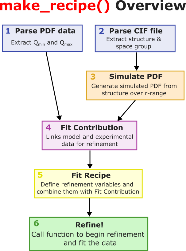

Parses PDF data: Given the PDF data file it extracts the Q_min and Q_max values.
Parses cif file: Given the cif file it extracts the structure and space group information.
Simulates a PDF: Given the structure, it computes a simulated PDF over predefined r-range.
Creates a Fit Contribution: This will hold the simulated PDF and the experimental PDF.
Creates a Fit Recipe: This is the main recipe that combines all contributions and parameters for the fit.
Refines params based on Fit Recipe: When the function is called, the parameters defined in the fit recipe are refined to best fit the data.

def make_recipe(cif_path, dat_path):

    # 1. Get structural info
    p_cif = getParser('cif') # Get the parser for CIF files
    stru = p_cif.parseFile(cif_path) # Using the parser, load the structure from the CIF
    sg = p_cif.spacegroup.short_name # Get the space group to constrain the fit later on

    # 2. Get PDF data
    profile = Profile() # Create a Profile object to hold PDF data and metadata
    parser = PDFParser() # Create a PDFParser to get the appropriate Q_min and Q_max
    parser.parseFile(dat_path) # Parse the PDF data file
    profile.loadParsedData(parser) # Load the parsed PDF data into the profile
    profile.setCalculationRange(
        xmin=PDF_RMIN, xmax=PDF_RMAX, dx=PDF_RSTEP
    )  # Set the calculation range for the PDF fit

    # 3. Create a PDFGenerator to generate a simulated PDF from the structure
    genpdf = PDFGenerator("generatedPDF") # Give the generator a name
    genpdf.setStructure(stru, periodic=True) # Give the generator the structure

    # 4. Create a Fit Contribution object
    contribution = FitContribution("niPDFfit") # Give the contribution a name
    contribution.addProfileGenerator(genpdf) # Add the PDFGenerator to the contribution

    # 5. Add the Profile to the contribution
    contribution.setProfile(profile, xname="r") # Add the Profile to the contribution

    # 6. Set the equation used to combine the simulated PDF with the experimental PDF
    contribution.setEquation("s1*generatedPDF") # scaling factor for the simulated PDF

    # 7. Create a Fit Recipe which turns our physics model into a mathematical recipe
    recipe = FitRecipe()
    recipe.addContribution(contribution) # Add the contribution to the recipe

    # 8. Initialize the experimental parameters
    recipe.niPDFfit.generatedPDF.qdamp.value = QDAMP_I
    recipe.niPDFfit.generatedPDF.qbroad.value = QBROAD_I
    recipe.niPDFfit.generatedPDF.setQmin(QMIN)
    recipe.niPDFfit.generatedPDF.setQmax(QMAX)

    # 9. Add scaling factor to the recipe
    recipe.addVar(contribution.s1, value=SCALE_I, tag="scale")

    # 10. Add structural params to recipe, constraining them to the space group
    spacegroupparams = constrainAsSpaceGroup(genpdf.phase, sg) # Extract SG constraints
    for par in spacegroupparams.latpars: # Iterate over constrained lattice parameters
        recipe.addVar(par,
                        value=CUBICLAT_I,
                        name="fcc_lat",
                        tag="lat")
    for par in spacegroupparams.adppars: # Iterate over constrained ADPs
        recipe.addVar(par,
                        value=UISO_I,
                        fixed=False,
                        name="fcc_ADP",
                        tag="adp")
    recipe.addVar(genpdf.delta2,
                    name="Ni_Delta2",
                    value=DELTA2_I,
                    tag="d2") # Add delta2 parameter for PDF peak broadening

    # 11. Add instrumental Qdamp and Qbroad parameters to the recipe
    recipe.addVar(genpdf.qdamp,
                    fixed=False,
                    name="Calib_Qdamp",
                    value=QDAMP_I,
                    tag="inst")
    recipe.addVar(genpdf.qbroad,
                    fixed=False,
                    name="Calib_Qbroad",
                    value=QBROAD_I,
                    tag="inst")
    return recipe

Now we can call make_recipe and plot the fit, experimental, and difference curves to evaluate how well the data fit.

recipe = make_recipe(cif_path, dat_path) # Call the function to create the fit recipe
recipe()
r = recipe.pdfcontrib.profile.x
g = recipe.pdfcontrib.profile.y
gcalc = recipe.pdfcontrib.profile.ycalc
diffzero = -0.65 * max(g) * np.ones_like(g) # offset the difference curve
diff = g - gcalc + diffzero

plt.figure(figsize=(15, 6))
plt.scatter(r, g, label="Experimental PDF")
plt.plot(r, gcalc, label="Fitted PDF")
plt.plot(r, diff, label="Difference")

plt.xlabel("r (Angstrom)")
plt.ylabel("G(r)")
plt.title("Ni PDF Fit")
plt.legend()
plt.show()

Once you run the above code, you should see a plot similar to the one below.

Congratulations! You have successfully fit a bulk Ni PDF using diffpy.cmi. You are now one step closer to becoming a PDF fitting expert.