Getting started

diffpy.stretched-nmf implements the stretched NMF algorithm for factorizing signal sets while accounting for uniform stretching along the independent axis.

Installation

The preferred method is conda:

conda config --add channels conda-forge
conda create -n diffpy.stretched-nmf_env diffpy.stretched-nmf
conda activate diffpy.stretched-nmf_env

For interactive plotting with show_plots=True, use a GUI-capable desktop environment. Conda installs use matplotlib-base, which is sufficient for plotting but still depends on an available interactive Matplotlib backend.

Alternatively, install from PyPI with pip:

pip install diffpy.stretched-nmf

For source installs (after cloning the repo):

pip install .

Quick check

Verify the CLI and Python import:

snmf --version
python -c "import diffpy.stretched_nmf; print(diffpy.stretched_nmf.__version__)"

Basic usage

The main entry point is the SNMFOptimizer class. Create an SNMFOptimizer with hyperparameters, then pass the source matrix to fit. The source matrix shape is (length_of_signal, number_of_signals).

import numpy as np
from diffpy.stretched_nmf.snmf_class import SNMFOptimizer

rng = np.random.default_rng(7)
source_matrix = rng.random((300, 24))  # (signal_length, n_signals)

snmf = SNMFOptimizer(
    n_components=3,
    max_iter=400,
    min_iter=20,
    tol=5e-7,
    rho=0,
    eta=0,
    random_state=7,
    show_plots=False,
)

snmf.fit(source_matrix=source_matrix, reset=True)

components = snmf.components_
weights = snmf.weights_
stretch = snmf.stretch_

Notes

• rho controls the stretching penalty (set to 0 for no stretching).

• eta controls sparsity (start at 0 and tune after selecting rho).

• Use reset=False only when you want to continue from the current solution.

XRD example

A complete real-data example is included in docs/examples/XRD_MgMnO_YCl_real.py. It reads the input matrices from docs/examples/data/XRD_MgMnO_YCl_real.

Run it from the repository root:

python docs/examples/XRD_MgMnO_YCl_real.py

The script runs a tuned XRD fit and writes my_norm_components.txt, my_norm_weights.txt, and my_norm_stretch.txt to the current working directory.

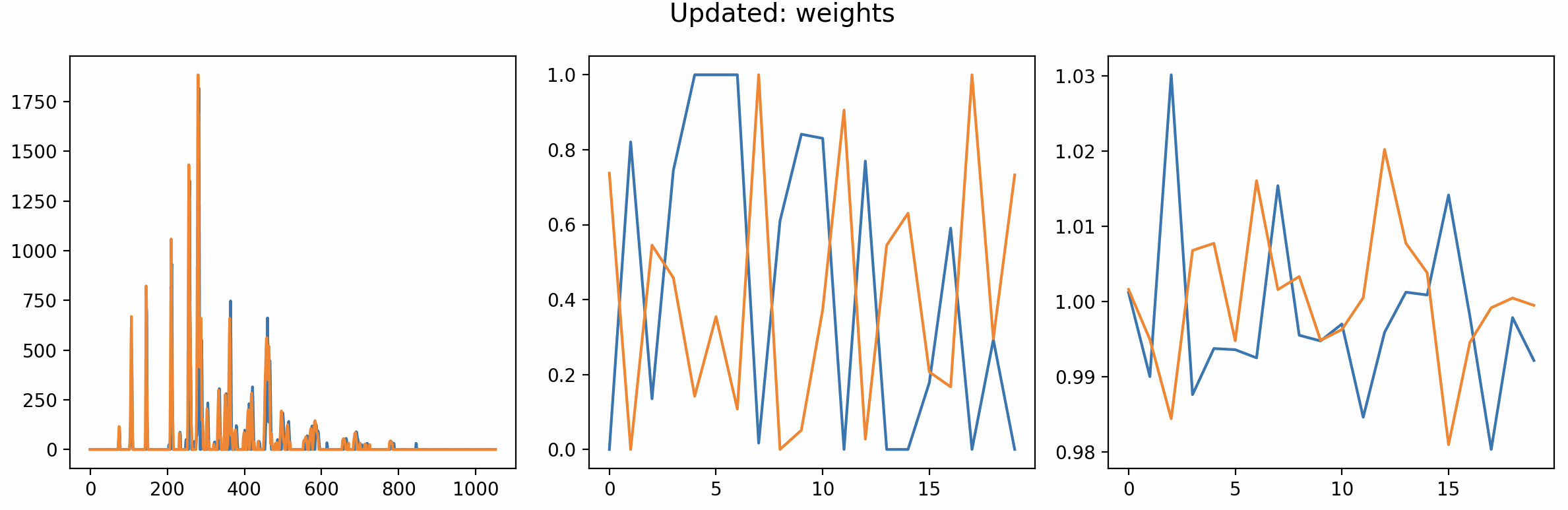
Preview from the show_plots interface from before the optimization has settled down.

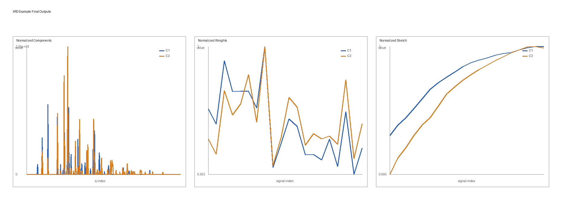
Final outputs: normalized components, normalized weights, and normalized stretch shown side by side.

Next steps

Browse the rest of the docs for release notes and license information.