Advanced Tutorials
diffpy.morph has some more functionalities not showcased in the quickstart tutorial.
Tutorials for these are included below. The files required for these tutorials can be downloaded
here.
For a full list of options offered by diffpy.morph, please run diffpy.morph --help on the command line.
Using MorphFuncxy
Examples of how to use the general morph MorphFuncxy with commonly used
diffraction software like PDFgetx3
and PyFai are directed to the
funcxy tutorials.
Performing Multiple Morphs
It may be useful to morph a PDF against multiple targets:
for example, you may want to morph a PDF against multiple PDFs measured
at various temperatures to determine whether a phase change has occurred.
diffpy.morph currently allows users to morph a PDF against all files in a
selected directory and plot resulting \(R_w\) values from each morph.
Within the
additionalDatadirectory,cdinto themorphsequencedirectory. Inside, you will find multiple PDFs of \(SrFe_2As_2\) measured at various temperatures. These PDFs are from “Atomic Pair Distribution Function Analysis: A primer”.Let us start by getting the \(R_w\) of
SrFe2As2_150K.grcompared to all other files in the directory. Rundiffpy.morph SrFe2As2_150K.gr . --multiple-targets
The multiple tag indicates we are comparing PDF file (first input) against all PDFs in a directory (second input). Our choice of file was
SeFe2As2_150K.grand directory was the cwd, which should bemorphsequence.
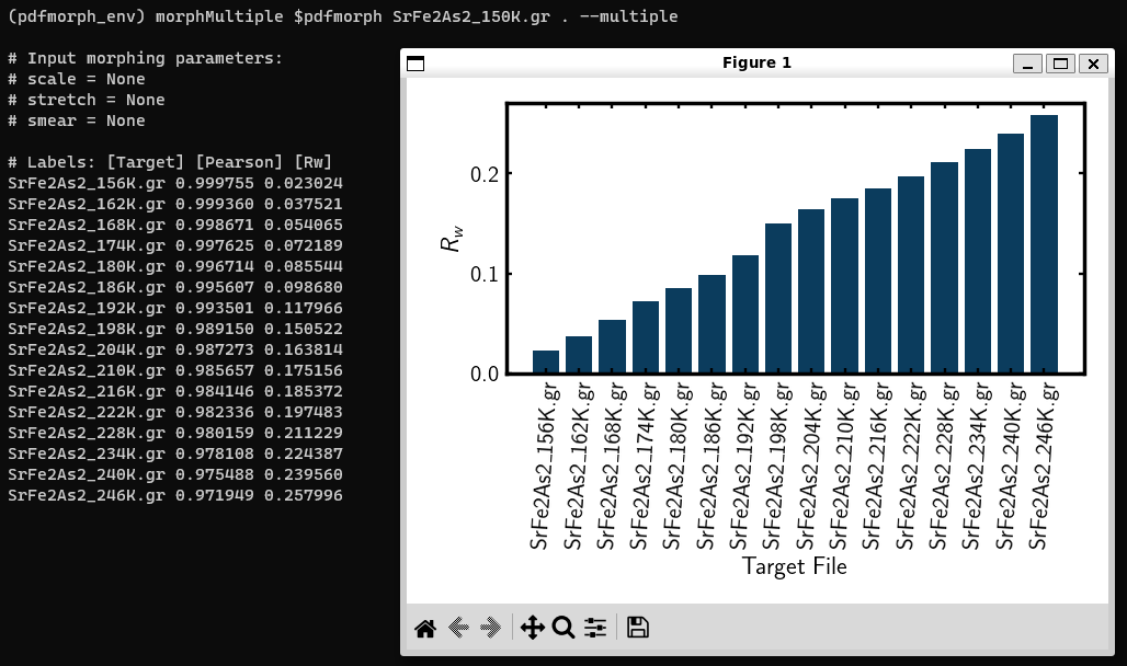
Bar chart of \(R_W\) values for each target file. Target files are listed in ASCII sort order.
After running this, we get chart of \(R_w\) values for each target file. However, this chart can be a bit confusing to interpret. To get a more understandable plot, run
diffpy.morph SrFe2As2_150K.gr . --multiple-targets --sort-by=temperature
This plots the \(R_w\) against the temperature parameter value provided at the top of each file. Parameters are entries of the form
<parameter_name> = <parameter_value>and are located above therversusgrtable in each PDF file.# SrFe2As2_150K.gr [PDF Parameters] temperature = 150 wavelength = 0.1 ...
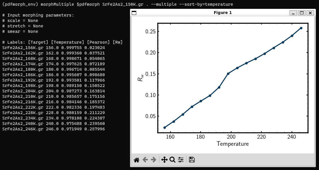
The \(R_W\) plotted against the temperature the target PDF was measured at.
Between 192K and 198K, the Rw has a sharp increase, indicating that we may have a phase change. To confirm, let us now apply morphs onto
SrFe2As2_150K.grwith all other files inmorphsequenceas targetsdiffpy.morph --scale=1 --stretch=0 SrFe2As2_150K.gr . --multiple-targets --sort-by=temperature
Note that we are not applying a smear since it takes a long time to apply and does not significantly change the Rw values in this example.
We should now see a sharper increase in \(R_w\) between 192K and 198K.
Go back to the terminal to see optimized morphing parameters from each morph.
On the morph with
SrFe2As2_192K.gras target,scale = 0.972085andstretch = 0.000508and withSrFe2As2_198K.gras target,scale = 0.970276andstretch = 0.000510. These are very similar, meaning that thermal lattice expansion (accounted for bystretch) is not occurring. This, coupled with the fact that the Rw significantly increases suggests a phase change in this temperature regime. (In fact, \(SrFe_2As_2\) does transition from orthorhombic at lower temperature to tetragonal at higher temperature!). More sophisticated analysis can be done with PDFgui.Finally, let us save all the morphed PDFs into a directory named
saved-morphs.diffpy.morph SrFe2As2_150K.gr . --scale=1 --stretch=0 --multiple-targets \ --sort-by=temperature --plot-parameter=stretch \ --save=saved-morphs
Entering the directory with
cdand viewing its contents withls, we see a file namedmorph-reference-table.txtwith data about the input morph parameters and re- fined output parameters and a directory namedmorphscontaining all the morphed PDFs. See the--save-names-fileoption to see how you can set the names for these saved morphs!
Polynomial Squeeze Morph
Another advanced feature in diffpy.morph is the MorphSqueeze morph,
which applies a user-defined polynomial to squeeze the morph function along the
x-axis. This provides a flexible way to correct for higher-order distortions
that simple shift or stretch morphs cannot fully address.
Such distortions can arise from geometric artifacts in X-ray detector modules,
including tilts, curved detection planes, or angle-dependent offsets, as well
as from intrinsic structural effects in the sample.
A first-order squeeze polynomial recovers the behavior of simple shift or stretch, while higher-order terms enable non-linear corrections. The squeeze transformation is defined as:
where \(a_0, a_1, ..., a_n\) are the polynomial coefficients defined by the user.
In this example, we show how to apply a squeeze morph in combination
with a scale morph to match a morph function to its target. The required
files can be found in additionalData/morphsqueeze/.
cdinto themorphsqueezedirectory:cd additionalData/morphsqueeze
Here you will find:
squeeze_morph.cgr— the morph function with a small built-in polynomial distortion.squeeze_target.cgr— the target function.
Suppose we know that the morph needs a quadratic and cubic squeeze, plus a scale factor to best match the target. As an initial guess, we can use:
squeeze = 0,-0.001,-0.0001,0.0001(for a polynomial: \(a_0 + a_1 x + a_2 x^2 + a_3 x^3\))scale = 1.1
The squeeze polynomial is provided as a comma-separated list (no spaces):
diffpy.morph --scale=1.1 --squeeze=0,-0.001,-0.0001,0.0001 -a squeeze_morph.cgr squeeze_target.cgr
diffpy.morphwill apply the polynomial squeeze and scale, display the initial and refined coefficients, and show the final differenceRw.To refine the squeeze polynomial and scale automatically, remove the
-atag if you used it. For example:diffpy.morph --scale=1.1 --squeeze=0,-0.001,-0.0001,0.0001 squeeze_morph.cgr squeeze_target.cgr
Check the output for the final squeeze polynomial coefficients and scale. They should match the true values used to generate the test data:
squeeze = 0, 0.01, 0.0001, 0.001scale = 0.5
diffpy.morphrefines the coefficients to minimize the residual between the squeezed, scaled morph function and the target.
Warning
Extrapolation risk:
A polynomial squeeze can shift morph data outside the target’s grid
(x-axis) range,
so parts of the output may be extrapolated.
This is generally fine if the polynomial coefficients are small and
the distortion is therefore small. If your coefficients are large, check the
plots carefully — strong extrapolation can produce unrealistic features at
the edges. If needed, adjust the coefficients to keep the morph physically
meaningful.
Experiment with your own squeeze polynomials to fine-tune your morphs — even small higher-order corrections can make a big difference!
Nanoparticle Shape Effects
A nanoparticle’s finite size and shape can affect the shape of its PDF.
We can use diffpy.morph to morph a bulk material PDF to simulate these shape effects.
Currently, the supported nanoparticle shapes include: spheres and spheroids.
Within the
additionalDatadirectory,cdinto themorphShapesubdirectory. Inside, you will find a sample Ni bulk material PDFNi_bulk.gr. This PDF is from “Atomic Pair Distribution Function Analysis: A primer”. There are also multiple.cgrfiles with calculated Ni nanoparticle PDFs.Let us apply various shape effect morphs on the bulk material to reproduce these calculated PDFs.
- Spherical Shape
The
Ni_nano_sphere.cgrfile contains a generated spherical nanoparticle with unknown radius. First, let us plotNi_blk.gragainstNi_nano_sphere.cgrdiffpy.morph Ni_bulk.gr Ni_nano_sphere.cgr
Despite the two being the same material, the Rw is quite large. To reduce the Rw, we will apply spherical shape effects onto the PDF. However, in order to do so, we first need the radius of the spherical nanoparticle.
To get the radius, we can first observe a plot of
Ni_nano_sphere.cgrdiffpy.morph Ni_nano_sphere.cgr Ni_nano_sphere.cgr
Nanoparticles tend to have broader peaks at r-values larger than the particle size, corresponding to the much weaker correlations between molecules. On our plot, beyond r=22.5, peaks are too broad to be visible, indicating our particle size to be about 22.4. The approximate radius of a sphere would be half of that, or 11.2.
Now, we are ready to perform a morph applying spherical effects. To do so, we use the
--radiusparameterdiffpy.morph Ni_bulk.gr Ni_nano_sphere.cgr --radius=11.2 -a --xmax=30
We can see that the \(Rw\) value has significantly decreased from before. Run without the
-atag to refinediffpy.morph Ni_bulk.gr Ni_nano_sphere.cgr --radius=11.2 --xmax=30
After refining, we see the actual radius of the nanoparticle was closer to 12.
Spheroidal Shape
The
Ni_nano_spheroid.cgrfile contains a calculated spheroidal Ni nanoparticle. Again, we can begin by plotting the bulk material against our nanoparticlediffpy.morph Ni_bulk.gr Ni_nano_spheroid.cgr
Inside the
Ni_nano_spheroid.cgrfile, we are given that the equatorial radius is 12 and polar radius is 6. This is enough information to define our spheroid. To apply spheroid shape effects onto our bulk, rundiffpy.morph Ni_bulk.gr Ni_nano_spheroid.cgr --radius=12 --pradius=6 -a --xmax=30
Note that the equatorial radius corresponds to the
--radiusparameter and polar radius to--pradius.Remove the
-atag to refine.
There is also support for morphing from a nanoparticle to a bulk. When
applying the inverse morphs, it is recommended to set --xmax=psize
where psize is the longest diameter of the nanoparticle.