Tutorial

In this tutorial we will convert several X-ray powder diffraction patterns to corresponding PDFs. Open a terminal on a Unix-based system or a Command Prompt on Windows and navigate to the examples folder included with the PDFgetX3 distribution. The examples folder can be found in the parent “doc” directory relative to this document or another option is to just search your file system for one of the input files mentioned below. The example files are also available at http://www.diffpy.org/doc/pdfgetx3/pdfgetx3-examples.zip.

Nickel X-ray PDF

predefined configuration file

Change to the Ni directory. The file named ni300mesh_300k_nor_1-5.chi contains powder X-ray data measured from nickel at the Advanced Photon Source beamline 6ID-D. The file contains two columns for the 2Θ scattering angles and X-ray intensities. The second file kapton_bgrd_300k_nor_2-3.chi contains the background measurement, i.e., the intensities from an empty capillary. Finally, the pdfgetx3.cfg contains a complete configuration parameters for converting the powder pattern to a PDF. Since all processing parameters are already defined in the configuration file, the first PDF calculation is very simple and involves running the pdfgetx3 program with the powder data file as an argument:

$ pdfgetx3 ni300mesh_300k_nor_1-5.chi

For the first run there should be no output on the screen, however a new file, ni300mesh_300k_nor_1-5.gr should appear in the work directory. We can use the plotdata program, installed with PDFgetX3, to plot the output data:

$ plotdata ni300mesh_300k_nor_1-5.gr

This will open a graph window and start an IPython interactive session. To exit and close the figure, type exit() on the IPython prompt. Let’s run the program again, but now with a --verbose=info option, to show more details about the program actions.

$ pdfgetx3 --verbose=info ni300mesh_300k_nor_1-5.chi

INFO:checking for environment variable PDFGETX3PATH
INFO:searching for default config file /home/user/.pdfgetx3.cfg
INFO:searching for default config file .pdfgetx3.cfg
INFO:searching for default config file pdfgetx3.cfg
INFO:loaded default config file pdfgetx3.cfg
INFO:parsing config file section [DEFAULT]
INFO:set config.dataformat = twotheta
INFO:set config.backgroundfile = kapton_bgrd_300k_nor_2-3.chi
INFO:set config.outputtypes = gr
INFO:set config.wavelength = 0.142774
INFO:set config.composition = Ni
INFO:set config.qmaxinst = 26.5
INFO:set config.qmax = 26.0
INFO:set config.rmin = 0.0
INFO:set config.rmax = 30.0
INFO:set config.rstep = 0.01
INFO:finished parsing config file
INFO:processing command line options
INFO:set config.verbose = info
INFO:finished with command line options
INFO:using 1 input files from the command line.
INFO:configuring PDFGetter mode 'xray'
INFO:calling config_xray
INFO:started PDF processing.
INFO:processing 'ni300mesh_300k_nor_1-5.chi'
INFO:resolved output file '' as 'ni300mesh_300k_nor_1-5.gr'
WARNING:ni300mesh_300k_nor_1-5.gr already exists.
WARNING:Use "--force=yes" or "--force=once" to overwrite.
INFO:elapsed time: 0.08

Here we can see what configuration files are searched, which of them get loaded and what are the effective values of the processing parameters. Unless the --verbose option is in effect, the program will show only messages that have either WARNING or ERROR importance. The warning line above indicates no output has been written, because that file already exists. This safety check can be overruled with the --force=yes option, upon which pdfgetx3 would overwrite any existing files.

PDFgetX3 output files start with a header that lists all the processing parameters and can be used as a valid configuration file with the -c option. Another option, --plot=[iq,sq,fq,gr] turns on plotting of the final PDF or of some other result. A side effect of the --plot option is that pdfgetx3 starts in an interactive mode, so the user can manipulate or save the plots. To put it all together, we are now going to redo the original PDF and plot its reduced total scattering function F(Q) and the PDF curve G(r). This time the chi file is not necessary, because the input file is already listed in the gr file that is now used as a custom configuration:

$ pdfgetx3 -c ni300mesh_300k_nor_1-5.gr --plot=fq,gr

WARNING:ni300mesh_300k_nor_1-5.gr already exists.
WARNING:Use "--force=yes" or "--force=once" to overwrite.

Variables related to PDF processing:

pdfgetter    -- PDFGetter used for calculation.
config       -- configuration data used by PDFGetter.
                See config.inputfiles for a list of inputs.
iraw         -- matrix of input raw intensities with 2 rows per file.
iq sq fq gr  -- intermediate results per each input file stored
                as matrix rows.

Functions:

tuneconfig   -- dynamically tune configuration variables.
processFiles -- process specified data files.
clearSession -- clear all elements from the inputfiles, iraw,
                iq, sq, fq and gr variables.
plotdata     -- plot all or selected columns from a text data file.
loadData     -- load all or selected columns from a text data file.
findfiles    -- search for files matching the specified patterns.

Use "%pdfgetx3" for a fresh run without exiting IPython.
In [1]:

This will open a plot figure similar to

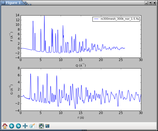
Because of the interactive mode implied by plotting, the program enters an IPython session. The IPython environment is preloaded with several extra functions and variables related to the PDF processing. For example, the config variable stores all the configuration parameters, and its content can be displayed with the print() function as

In [1]: print(config)

args = ['-c', 'ni300mesh_300k_nor_1-5.gr', '--plot=fq,gr']
configfile = ni300mesh_300k_nor_1-5.gr
...
qmax = 26.0
...

The processFiles() function allows to redo the whole calculation and plotting process for additional input files or for new parameter values. To plot the F(Q) and G(r) curves calculated at Q_max = 22 Å^-1, we can call processFiles() and pass it a keyword argument for the new qmax as follows:

In [2]: processFiles(qmax=22)

# the qmax parameter was updated to a new value, thus
In [3]: config.qmax
Out[3]: 22

There should be now two lines in each plot axis corresponding to the results at Q_max equal 26 and 22 Å^-1. To exit the program, type exit().

processing from scratch

We have already encountered the command-line option -c for specifying a custom configuration file. A special argument “NONE”, will make pdfgetx3 ignore any configuration files and start up in a default state. We can use this feature to process the nickel PDF as if we did not have any configuration file:

$ pdfgetx3 -c NONE ni300mesh_300k_nor_1-5.chi

WARNING:Nothing to do, use "-t" or "--plot" options.
ERROR:Configuration error: wavelength not specified.
ERROR:See "--help" for more hints.

There is an error, for the wavelength is necessary to convert the scattering angle 2Θ to momentum transfer Q. The X-ray wavelength was 0.142774 Å, which can be passed with the -w, --wavelength option:

$ pdfgetx3 -c NONE ni300mesh_300k_nor_1-5.chi -w 0.142774

...
ERROR:Configuration error: Chemical composition not known.
ERROR:See "--help" for more hints.

There is still an error. The PDF calculation needs an average X-ray scattering factor of the material, which is obtained from sample chemical composition. The composition can be specified with the --composition option. The example below uses a “\” character to indicate the command continues on the next line. Such syntax works in Unix terminals, but on Windows the command has to be typed all on a single line:

$ pdfgetx3 -c NONE ni300mesh_300k_nor_1-5.chi -w 0.142774 \
           --composition=Ni

WARNING:Nothing to do, use "-t" or "--plot" options.
...

There was no error message this time, but the program complains about a lack of action. The pdfgetx3 program does not write any results unless instructed by the -t, --outputtypes option. The outputtypes option recognizes the following result types: “iq”, “sq”, “fq”, “gr”. One or more of these type strings, separated by a comma, can be included with the -t option, which will produce the corresponding output files. An empty string, such as -t "", or -t NONE may be used to clear any outputtypes defined in the configuration file, and avoid the unseemly file-exists warnings.

At this point, we will not write any output files, but will use the --plot option to display the calculated curves. The --plot accepts the same arguments as outputtypes, so to display the F(Q) and G(r) curves we shall run

$ pdfgetx3 -c NONE ni300mesh_300k_nor_1-5.chi -w 0.142774 \
           --composition=Ni --plot=fq,gr

WARNING:qmaxinst reset to last nonzero point qmaxinst=28.0865680161
WARNING:qmax reset to the data boundary qmaxinst=28.0865680161

which should open the following plot window:

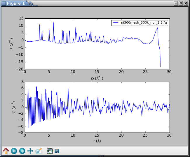
The graphs look terrible. The PDF is very noisy and the F(Q) curve shows a sudden break at about 27 Å^-1. What happened? The powder intensities are inaccurate at a very top of the detector angular range. The interactive session is setup with iraw, iq, sq, fq, gr variables for the original raw data and intermediate results. We are going to plot the “iq” variable that has the input intensities resampled on the Q grid. The matplotlib function clf() clears the figure, the iq variable is a two-row matrix with Q and I rows, and the axis() function lets us zoom to a given range:

In [1]: clf()
In [2]: plot(iq[0], iq[1])
Out[2]: [<matplotlib.lines.Line2D at 0x3e20f50>]
In [3]: axis([20, 29, 0, 3000])
Out[3]: [20, 29, 0, 3000]

The graph shows a sudden drop in the raw intensities at 27 Å^-1. The qmaxinst variable defines a Q cutoff for a meaningful instrument intensities and, to be on a safe side, we are going to set it to 26.5 Å^-1

In [4]: processFiles(qmaxinst=26.5)
WARNING:qmax reset to the data boundary qmaxinst=26.5

The updated curves looks reasonable without any oscillations and breakpoints. The tuneconfig() function provides a GUI-driven way for visualizing the processing parameters and their effect on the results. Type tuneconfig() to execute the function, which should open a new window with several sliders. Try to move different sliders and see how do the F(Q) and G(r) curves change. The rpoly parameter controls the degree of data-correction polynomial and is an approximate low-r bound of reliable G values. Once the parameters are tuned, they may be set to exact values. We will also turn on the writing of the G(r) curve and save it to an output file nicmd.gr:

In [14]: config.qmax = 26
In [15]: config.outputtypes = 'gr'
In [16]: config.output = 'nicmd'
In [17]: processFiles()

Platinum data series

PDFgetX3 has been designed to handle large series of data files. With the fast area-detectors it is easy to measure hundreds of X-ray patterns in a time or temperature series. Normally, these input files need to be entered as command line arguments to the pdfgetx3 program. This is usually no problem with Unix-like shells, which expand filename patterns to a list of matching files. However, such file generation is in general not available on Windows. The input file names tend to include scan numbers which are useful for selecting desired data, yet even with Unix shells it is difficult to match a range of scan numbers (z-shell being a notable exception).

matching input files

The pdfgetx3 program includes a built-in function for finding a set of input files. The command line arguments are normally taken as input file names. However, if the -f, --find option is present, the arguments are understood as patterns and the program looks for files that match ALL of them. Another option -l, --list makes pdfgetx3 print out the matching files without any other action, which can be used to verify if the patterns match intended files.

We will try out this file search on platinum example files. Open a terminal and navigate to the Pt directory. There should be a series subdirectory with 6 chi files indexed from 903 to 908. At first, let’s stay in the Pt directory and run the following command

$ pdfgetx3 --list --find

Pt_bulk-00055-pdfgetx2.gr
Pt_bulk-00055-pdfgetx3.gr
Pt_bulk-00055.chi
Pt_bulk-00055.gr
empty_capillary-00032.chi
pdfgetx3.cfg
plotpdfcomparison.py

Without any patterns the file search matches all files in the current directory. Now let’s try to add name patterns. There are few special patterns, for example ^ matches at the beginning of the filename, $ at the end and <N-M> matches a range of integer values from N to M. The patterns containing ^$<> need to be quoted as these characters have special meaning in the shell. Here are some examples how it works.

Filenames containing “y”:

$ pdfgetx3 --list --find y
empty_capillary-00032.chi
plotpdfcomparison.py

Filenames that containing both “y” and “chi”, here we use the options --list and --find in an abbreviated form -l and -f:

$ pdfgetx3 -lf y chi
empty_capillary-00032.chi

Filenames that start with “e”:

$ pdfgetx3 --list --find "^e"
empty_capillary-00032.chi

Filenames that contain character “2”:

$ pdfgetx3 --list --find 2
Pt_bulk-00055-pdfgetx2.gr
empty_capillary-00032.chi

Filenames that contain numeric value “2”:

$ pdfgetx3 -lf "<2>"
Pt_bulk-00055-pdfgetx2.gr

data search path

PDFgetX3 can be run with the -d, --datapath option, which tells it to search additional directories for input data files. The -d option can be used several times to search more directories. The data directories can be also defined with the PDFGETX3PATH environment variable. Here we will use the -d option to match files in the series subdirectory. The search stops at the first directory that contains any match, therefore

$ pdfgetx3 --datapath=series --list --find Pt chi
Pt_bulk-00055.chi

matches just one file in the current working directory, but

$ pdfgetx3 --datapath=series --list --find Pt "<906->.chi"
series/Pt_bulk_ramp03-00906.chi
series/Pt_bulk_ramp03-00907.chi
series/Pt_bulk_ramp03-00908.chi

finds 3 files, because only the series folder contains file names with “Pt” and a number “906” or higher followed by “.chi”.

output file names

By default the output files are saved in the current directory. The output path, can be changed with the -o, --output option. The -o recognizes several aliases that are replaced with parts of the input file name, for example, “@b” expands to an extension-stripped base name. In similar faction, “@o” is replaced with the output type extension. Thus to generate PDFs for all files in the series directory and save them in the series-gr subfolder do

$ pdfgetx3 -d series --find "<900-910>.chi" --output=series-gr/@b.@o

The extension “.@o” is automatic when not included anywhere in the output file name. Thus to process the Pt series at Q_max = 18 Å^-1 while saving the results in the same folder, but with “qmax18” in their filename can be done with:

$ pdfgetx3 -d series --find "<900-910>.chi" --qmax=18 -o series-gr/@b_qmax18

The series-gr directory should now contain 12 gr files, 6 of them processed at the Q_max = 27 Å^-1 from the configuration file and 6 other at Q_max = 18 Å^-1.

Interactive tuning of parameters

One of the most powerful features of PDFgetX3 is the ability to tune PDF processing parameters in an interactive mode and immediately visualize their effect on the results. To demonstrate this feature, navigate to the examples/Ni directory in the shell and process the nickel PDF while plotting the F(Q) and G(r) curves. Because of plotting the program will open an interactive IPython session. The tuning mode can be then entered by calling the tuneconfig() function from the IPython environment

$ pdfgetx3 --plot=fq,gr ni300mesh_300k_nor_1-5.chi
...
In [1]: tuneconfig()

The tuneconfig() function will by default add a second set of live lines for the plotted curves and open a GUI dialog with sliders for the tunable process parameters. Changing any slider would immediately recalculate the PDF and update live lines in the plot.

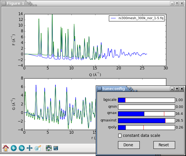
The constant data scale check-box rescales the result curves to a constant maximum value. This is useful for assessing if a parameter change produces different curve shape or if it just rescales the results. The tunable parameters are described in the PDF parameters section. Only the active parameters are displayed in the tuneconfig GUI, thus there would be no slider for the bgscale parameter if PDF has been processed without any background data.

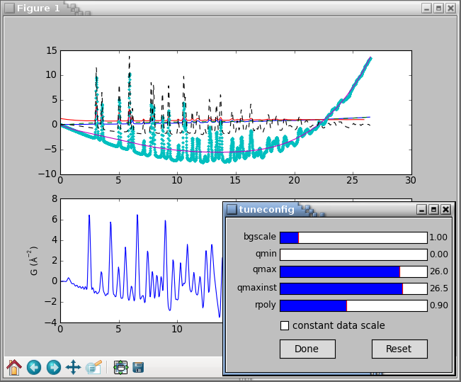
By default the tuneconfig() function displays the same curves as specified by the --plot option, however it can be configured to show arbitrary intermediate results or even visualize selected steps in the PDF processing. We shall demonstrate this by showing a live-plot of the polynomial correction together with the final PDF. At first, we shall use the describe() method of the pdfgetter() object to print out the chain of transformations involved in the PDF processing and obtain a reference to the transformation object t4 that applies the polynomial correction. The transformation object can be then included in a list of plot identifiers that are passed to the tuneconfig() function

$ pdfgetx3 --plot=fq,gr ni300mesh_300k_nor_1-5.chi
...
Use "%pdfgetx3" for a fresh run without exiting IPython.

In [1]: clf()
In [2]: pdfgetter.describe()
0   TransformTwoThetaToQA
    convert x data from twotheta to Q in 1/A
1   TransformQGridRegular
    Remove the data outside the (qmin, qmaxinst) range
2   TransformBackground
    subtract background intensity
3   TransformXrayASFnormChris
    scale and normalize intensities by x-ray scattering factors
4   TransformSQnormRPoly
    Normalize S(Q) by fitting a polynomial
5   TransformSQToFQ
    Convert S(Q) to F(Q).
6   TransformFQgrid
    Resample F(Q) to a regular grid suitable for FFT
7   TransformFQToGr
    Convert F(Q) to G(r).
In [3]: t4 = pdfgetter.getTransformation(4)
In [4]: tuneconfig([t4, 'gr'])

The clf() function used above clears the figure to remove the initial F(Q) line from the first panel. Overall, this should display the following plot:

The tuning can be finished by clicking the Done button or closing the tuneconfig GUI window. The parameter values can be thereafter adjusted to a rounded values by setting an attribute of the config object, for example:

In [5]: config.bgscale = 1.5

Finally, to save the new results, we shall first confirm outputtypes have been correctly set and then use the processFiles() function to redo the calculations, plots and data output for the updated configuration. Note that the processFiles() function accepts keyword arguments for configuration parameters. This is used at line In [8] to turn on the force flag and is in effect a shortcut for an extra config.force = True statement.

In [6]: config.outputtypes
Out[6]: ['gr']
In [7]: processFiles()
WARNING:ni300mesh_300k_nor_1-5.gr already exists.
WARNING:Use "--force=yes" or "--force=once" to overwrite.
In [8]: processFiles(force=True)

ni300mesh_300k_nor_1-5.gr was successfully saved at an updated configuration for there were no warnings after the last call.